
Fluid Dynamics#
Author:
Date:
Time spent on this assignment:
import numpy as np
import matplotlib.pyplot as plt
import math
from matplotlib.animation import FuncAnimation
import itertools
from IPython.display import HTML
import pickle

def reset_me(keep_list=[]):
    """Reset the notebook namespace, preserving selected variables.

    Inputs:
        keep_list (list[str]): names of variables to keep in the namespace.
    """
    ll = %who_ls
    keep_list = keep_list + ['reset_me', 'np', 'plt', 'math', 'FuncAnimation',
                             'HTML', 'itertools', 'pickle', 'test_func']
    for iiii in keep_list:
        if iiii in ll:
            ll.remove(iiii)
    for iiii in ll:
        jjjj = "^" + iiii + "$"
        %reset_selective -f {jjjj}
    ll = %who_ls
    return

def test_func(func, in_files, out_files):
    """Test ``func`` by loading pickled inputs from "in_files" and comparing to expected outputs.

    Inputs:
        func (callable): the function to test.
        in_files (list[str]): paths to pickle files holding the inputs to ``func``.
        out_files (list[str]): paths to pickle files holding the expected outputs.
    """
    inputs  = [pickle.load(open(f, "rb")) for f in in_files]
    outputs = [pickle.load(open(f, "rb")) for f in out_files]
    result  = func(*inputs)
    all_good = True
    if not isinstance(result, tuple):
        result = (result,)
    for i in range(len(outputs)):
        if np.max(np.abs(result[i] - outputs[i])) > 1e-14:
            print("Failed test for", out_files[i], i, np.max(np.abs(result[i] - outputs[i])))
            all_good = False
    if all_good:
        print("Test Passed!")
    else:
        print("Test Failed :(")
Download the test files here, or download them from the website and upload & unzip them to wherever this notebook file is.
!wget https://courses.physics.illinois.edu/phys246/fa2020/code/TestFiles.zip && unzip TestFiles.zip
Python Warmup#
Useful functions:#
Before we begin, we want to highlight some functions that you may find useful in this assignment. We’ll explore the last one in more depth as well.
np.zeros([dimensions])- create an array filled with all zeros. *Ex:n = np.zeros([9,10,10])creates a (9,10,10) array of all zeros.np.ones([dimensions])- same thing asnp.zerosbut with all ones.np.empty([dimensions])- same thing asnp.zerosbut fills array with garbage. Very fast compared to the above.np.roll(x,shift,axis)- shift arrayxbyshiftalongaxis.
Warmup - using np.roll#
Something we’ll see later in this assignment is the need to shift elements right, left, up, down, and diagonally. Let’s make a little test problem to illustrate how this works.
# Run me!
x = np.arange(15).reshape(3,5)
print(x)
[[ 0  1  2  3  4]
 [ 5  6  7  8  9]
 [10 11 12 13 14]]
Now we’ll want to shift every element in x to the right, wrapping everything around the edge. Rather than figuring this out with a for loop, we’ll employ np.roll to do it quickly.
print(x,'\n')
print(np.roll(x,(0,1),(0,1)))
[[ 0  1  2  3  4]
 [ 5  6  7  8  9]
 [10 11 12 13 14]]

[[ 4  0  1  2  3]
 [ 9  5  6  7  8]
 [14 10 11 12 13]]
Now let’s dissect that command. The first (0,1) means don’t shift the “y” direction, and shift the “x” direction by +1. The next argument, which should always be (0,1), means to apply the shift as a (row, column) matrix.
Now let’s go left:
print(x,'\n')
print(np.roll(x,(0,-1),(0,1)))
[[ 0  1  2  3  4]
 [ 5  6  7  8  9]
 [10 11 12 13 14]]

[[ 1  2  3  4  0]
 [ 6  7  8  9  5]
 [11 12 13 14 10]]
🦉 Now we’ll try to implement a section of the Cha-Cha Slide(Lyrics)
♫Now it's time to get funky
To the right now, to the left
Take it back now y'all♪
Make your x array go right, then left, then “down”. Your output should be:
[[ 4  0  1  2  3]
 [ 9  5  6  7  8]
 [14 10 11 12 13]]
[[ 1  2  3  4  0]
 [ 6  7  8  9  5]
 [11 12 13 14 10]]
[[ 5  6  7  8  9]
 [10 11 12 13 14]
 [ 0  1  2  3  4]]
(Notice how down isn’t what you may expect…)
#!Start
print(np.roll(x,(0,1),(0,1)))
print(np.roll(x,(0,-1),(0,1)))
print(np.roll(x,(-1,0),(0,1)))
#!Stop
[[ 4  0  1  2  3]
 [ 9  5  6  7  8]
 [14 10 11 12 13]]
[[ 1  2  3  4  0]
 [ 6  7  8  9  5]
 [11 12 13 14 10]]
[[ 5  6  7  8  9]
 [10 11 12 13 14]
 [ 0  1  2  3  4]]
🦉In a special version of the song, the next line goes
♫ Take it diagonally up and to the right now y'all
Implement this array move, you should get:
[[14 10 11 12 13]
 [ 4  0  1  2  3]
 [ 9  5  6  7  8]]
print(np.roll(x,(1,1),(0,1))) #!#
[[14 10 11 12 13]
 [ 4  0  1  2  3]
 [ 9  5  6  7  8]]
Now you’re a ~~Cha-Cha Slide~~ np.roll master!
Exercise 1: Fluid Dynamics#
List of collaborators:
References you used in developing your code:
In this assignment you will produce a fluid dynamics simulation. Our simulation is based on the lattice Boltzmann method. We will describe the microscopic behavior of the fluid using a 9-component model on a grid, which will be called n.
Each of the 9 components represents a density of fluid moving in a different direction: stationary, up, down, left, right, and each of the diagonal directions. Propagation forward in time consists of three main steps:
Boundary conditions – In our case, we will assume periodic boundary conditions in the y direction (imagine a fluid in a torus), constant flow on the left, and smooth flow on the right.
Relaxation/collision – If some bits of fluid are moving right and some are moving left, they collide with each other at a certain rate.
Propagation/moving – Fluid that is moving right will move right and so on, and fluid bounces off any obstacles.
The macroscopic quantities density \(\rho\) and overall velocity u just by summing up the amount and velocities of the microscopic fluid components in n.
We are going to develop a number of functions which you will store in the cell below (as well as some global variables that we will use throughout this exercise).
Note that the only global variables you should ever use are constants, which in this exercise are nx,ny, and the velocities directions for each of the components v. Because they do not change in the entire workbook, it is reasonably safe to declare them as global variables.
The global variables are
nx=520; ny=180 #size of our simulation

### ANSWER HERE

If you have a function that takes in an array n, always make a new variable to return. This will allow you to compose functions, so that you can call f(g(n)) which will apply g to n and then f to the output of g.
def do_math(n):
    n[0,2] = 5 # this modifies n in place so the argument will also change. You don't want that.
    # instead, do
    nout = n.copy()
    nout[0,2] = 5
    nout = 2*n+5 # this makes a new object automatically
    return nout
a. Making some obstacles#
To simulate the real world on the computer, we’ll break the tunnel into \(n_x \times n_y\) squares which we’ll call voxels.
Your simulation will be doing fluid dynamics in an \(n_x \times n_y\) “tunnel” which has some objects within it. These objects will be represented by a boolean \(n_x \times n_y\) size array obstacle=np.empty((nx,ny),dtype='bool') which should be True where the obstacle is and False otherwise. For example,
obstacle[:,:]=False
obstacle[50:70,50:70]=True
This would set up a square \(20 \times 20\) object inside our tunnel.
🦉Add a generate_cylinder_obstacle() function to the “function-cell” above which generates an object which is a cylinder located at \((n_x/4,n_y/2)\) with a radius of \(n_y/9\)
You can test it by calling
plt.matshow(generate_cylinder_obstacle().transpose())
plt.xlabel("")
plt.ylabel("")
plt.title("put title here")
It should look like this

Docstring specification:
def generate_cylinder_obstacle():
    """Build a boolean obstacle mask containing a single cylinder.

    Returns:
        obstacle (np.ndarray[bool], shape (nx, ny)): ``True`` inside a disk of
        radius ``ny/9`` centered at ``(nx/4, ny/2)``; ``False`` elsewhere.
    """
object as a variable! Notice how
object is green in a cell - this means it is a special keyword.### ANSWER HERE
b. Microscopic velocities \(v_i\)#
To simulate the real world on the computer, we’ll break the tunnel into \(n_x \times n_y\) squares which we’ll call voxels.
The key quantity in your simulation is nine microscopic degrees of freedom
\(n_k(i,j)\) where \(0\leq k \leq 8\) and \((i,j)\) are over the \(n_x \times n_y\) voxels of your simulation
which are going to be nine different densities (for each voxel \((i,j)\)) which correspond to the density of a fluid at \((i,j)\) moving in nine different directions (or velocities \(v_k\)):
\(n_0\): stationary fluid moving at velocity \(v_0=(0,0)\)
\(n_1\): fluid moving up moving at velocity \(v_1=(0,1)\)
\(n_2\): fluid moving down at velocity \(v_2=(0,-1)\)
\(n_3\): fluid moving right at velocity \(v_3=(1,0)\)
\(n_4\): fluid moving left at velocity \(v_4=(-1,0)\)
\(n_5\): fluid moving left-down at velocity \(v_5=(-1,-1)\)
\(n_6\): fluid moving left-up at velocity \(v_6=(-1,1)\)
\(n_7\): fluid moving right-down at velocity \(v_7=(1,-1)\)
\(n_8\): fluid moving right-up at velocity \(v_8=(1,1)\)
It will be useful to have access to these microscopic velocities as global variables. 🦉Go ahead and add to the top of your “function-cell” the various velocities:
v=np.zeros((9,2),dtype='int')
v[0,:]=[0,0]
v[1,:]=[0,1]
...
Plot these (below) as
for i in range(0,9):
    plt.arrow(0,0,v[i,0],v[i,1],head_width=0.05, head_length=0.1, fc='k', ec='k')
plt.xlim(-1.2,1.2)
plt.ylim(-1.2,1.2)
plt.show()
and make sure it looks like

### ANSWER HERE
We will represent the microscopic densities by a variable
n=np.zeros(9,nx,ny)
The high level algorithm for fluid dynamics is very simple. After setting up the initial conditions, we loop many times doing
Adjust boundary conditions
Collide the microscopic densities
Move the microscopic densities
c. Computing macroscopic quantities from the microscopic density#
Given the microscopic densities, there are two macroscopic quantities:
the macroscopic density \(\rho(i,j)=\sum_k n_k\) (size: \(n_x \times n_y\))
the macroscopic velocity \(\vec{u}(i,j) \equiv (u_x(i,j),u_y(i,j))\) (size: \(2 \times n_x \times n_y\)) where
\(u_x(i,j) = 1/\rho \sum_k v_{k,x} n_k(i,j)\)
\(u_y(i,j) = 1/\rho \sum_k v_{k,y} n_k(i,j)\)
which you will compute using the function (you will write) (rho,u) = micro_to_macro(n)
🦉Go ahead and write this function and add it to your ‘function-cell’
You can test it using these lines of code:
test_func(micro_to_macro,["Microscopic.dat"],["rho_after_Micro2Macro.dat","u_after_Micro2Macro.dat"])
and see if it prints two zeros (which is a success!).
If you have trouble, you can get the expected output by calling for example:
in_array = pickle.load(open("Microscopic.dat", "rb"))
ref_rho = pickle.load(open("rho_after_Micro2Macro.dat", "rb"))
calc_rho, calc_u = micro_to_micro(in_array)
# plot calc_rho and calc_u
Docstring specification:
def micro_to_macro(n):
    """Compute macroscopic density and velocity from microscopic densities.

    Inputs:
        n (np.ndarray, shape (9, nx, ny)): microscopic densities for the nine
            lattice directions.

    Returns:
        rho (np.ndarray, shape (nx, ny)): macroscopic density.
        u   (np.ndarray, shape (2, nx, ny)): macroscopic velocity (ux, uy).
    """
Tip: Because u is \((2,n_x,n_y)\), we can get ux by doing u[0] (which is then a \((n_x,n_y)\) array) and uy by doing u[1].
optional - np.einsum#
Figuring out the summations efficiently can be a pain, but we can use np.einsum help out here. Figure out how to rewrite the above problem with Einstein summation notation. To use the function, if we have
$\(
A_{ijk}\cdot B_{dk} = C_{ijd},
\)$
we’d then call:
C = np.einsum("ijk,dk->ijd",A,B)
##ANSWER HERE
d. Getting the equilibrium microscopic densities.#
Given the macroscopic densities \(\rho\) and \(\vec{u}\), there are equilibrium microscopic densities \(n_{eq}\) (size: \(9 \times n_x \times n_y\)) which you will compute using n_eq=macro_to_equilibrium(rho,u)
The relevant formula for this is
where
\(\omega_{0}=4/9\)
\(\omega_{1-4}=1/9\)
\(\omega_{5-8}=1/36\)
Given some microscopic densities \(n\) you should be able then to figure out the equilibrium microscopic densities \(n_{eq}\).
🦉Write the function macro_to_equilibrium, adding it to your “function-cell”.
You can test it by checking if
test_func(macro_to_equilibrium,["rho_after_Micro2Macro.dat","u_after_Micro2Macro.dat"],["Microscopic_after_equilibrium.dat"])
is equal to zero.
Docstring specification:
def macro_to_equilibrium(rho, u):
    """Compute the equilibrium microscopic densities from macroscopic fields.

    Inputs:
        rho (np.ndarray, shape (nx, ny)): macroscopic density.
        u   (np.ndarray, shape (2, nx, ny)): macroscopic velocity field.

    Returns:
        n_eq (np.ndarray, shape (9, nx, ny)): equilibrium microscopic densities.
    """
### ANSWER HERE
d. Implementing collision#
Once you can compute these quantities, the next step is to implement the collision step.
🦉Write a function collision(n,obstacle) which returns the density n after collision. Put it in your function-cell above.
When we collide the microscopic densities, we get new microscopic densities given as
nout = n * (1-omega) + omega * neq
Here are the steps for the function: \(\phantom{}\)
Calculate
neq
a. take the microscopic densities \(\rightarrow\) compute the macroscopic density and velocity(rho,u) = micro_to_macro(n)
b. take the macroscopic density and velocity \(\rightarrow\) compute the equilibrium microscopic densitiesneq=macro_to_equilibrium(rho,u)Calculate
nout = n * (1-omega) + omega * neq
a. \(\omega\) is the viscosity parameter. We will use \(\omega =1.9572953736654806\)We moved fluid where the obstacle is, so we need to undo this. Reset all
noutwhere the obstacle is to be the same asn
Test with
test_func(lambda x: collision(x,generate_cylinder_obstacle()),["Microscopic.dat"],["Microscopic_after_collision.dat"])
Docstring specification:
def collision(n, obstacle):
    """Apply one collision/relaxation step to the microscopic densities.

    Inputs:
        n (np.ndarray, shape (9, nx, ny)): microscopic densities.
        obstacle (np.ndarray[bool], shape (nx, ny)): obstacle mask.

    Returns:
        n_out (np.ndarray, shape (9, nx, ny)): densities after collision,
        with obstacle voxels left unchanged.
    """
### ANSWER HERE
e. Moving#
We’ll now move on to getting the fluid to move. This will be a function called, surprise, move(n,obstacle). But first we need two helper functions:
bounce(n,obstacle)bounce the velocities – that is, every velocity where the obstacle is gets reversed
move_density(n)Move all your densities in the direction of the velocity (hint the velocity tells you where to move it)
Assume periodic boundary conditions here
🦉 Implement bounce(n,obstacle) -> nout
bounce the velocities off the obstacle – every velocity where the obstacle is gets reversed
Docstring specification:
def bounce(n, obstacle):
    """Reverse velocities at every voxel occupied by the obstacle.

    Inputs:
        n (np.ndarray, shape (9, nx, ny)): microscopic densities.
        obstacle (np.ndarray[bool], shape (nx, ny)): obstacle mask.

    Returns:
        n_out (np.ndarray, shape (9, nx, ny)): densities with directions
        flipped inside the obstacle.
    """
## ANSWER HERE
🦉 Implement move_density(n) -> n
Move all your densities in the direction of the velocity (hint the velocity tells you where to move it)
Assume periodic boundary conditions here
🦉 Test using
test_func(move_density,["Microscopic.dat"],["Microscopic_after_moveDensity.dat"])
Docstring specification:
def move_density(n):
    """Propagate each density component in its own velocity direction.

    Inputs:
        n (np.ndarray, shape (9, nx, ny)): microscopic densities.

    Returns:
        n_out (np.ndarray, shape (9, nx, ny)): densities after propagation
        with periodic boundary conditions.
    """
## ANSWER HERE
move(n,obstacle) call is just a bounce then move_density.
🦉Write this function and test!
test_func(lambda x: move(x,generate_cylinder_obstacle()),["Microscopic.dat"],["Microscopic_after_move.dat"])
Docstring specification:
def move(n, obstacle):
    """Combine :func:`bounce` and :func:`move_density` into a single move step.

    Inputs:
        n (np.ndarray, shape (9, nx, ny)): microscopic densities.
        obstacle (np.ndarray[bool], shape (nx, ny)): obstacle mask.

    Returns:
        n_out (np.ndarray, shape (9, nx, ny)): densities after bouncing
        off the obstacle and propagating.
    """
### ANSWER HERE
f. Boundary conditions#
In the y-direction, we’ll assume periodic boundary conditions. For the x-direction, we’ll assign specific boundary conditions on the left and right.
Let’s call this function fix_boundary(n,n_init) which applies these boundary conditions and returns the new density n.
Left: we assume there is a constant inflow – the microscopic densities are the same at each step. Therefore, we simply replace the current densities on the left-most row with the initial microscopic densities (n_init).
Right: we assume the gradient is zero – i.e., the important physics has disappeared by this point. To do this, we set
# loop over all microscopic velocities vL that are going left
   nout[vL,-1,:] = nout[vL,-2,:]
Hint: there are 3 vLs.
🦉Put all of this together and run the next test!
Testing:
test_func(fix_boundary,["Microscopic.dat","Microscopic2.dat"], ["Microscopic_after_boundary.dat"])
Docstring specification:
def fix_boundary(n, n_init):
    """Apply left-inflow and right-zero-gradient boundary conditions.

    Inputs:
        n (np.ndarray, shape (9, nx, ny)): current microscopic densities.
        n_init (np.ndarray, shape (9, nx, ny)): initial microscopic densities
            that set the left boundary inflow.

    Returns:
        n_out (np.ndarray, shape (9, nx, ny)): densities after applying
        the x-boundary conditions.
    """
### ANSWER HERE
g. Setting up the initial conditions#
We need to generate initial conditions. The way that we are going to do that is
pick some macroscopic density \(\rho\) of size \((n_x,n_y)\) (uniformly equal to 1.0) and a
macroscopic velocity \(\vec{u}(i,j)\) (sizes \((2,n_x,n_y)\))
0.04*(1.0+1e-4*np.sin(y/(ny)*2*np.pi))in the x-direction (aka 0). This introduces a very tiny anisotropy to the system.zero in the y-direction (aka 1)
compute the equilibrium density \(n_{eq}\) associated with the initial density and velocities.
Use (and return) this as the initial conditions
🦉Write a function setup() which returns the initial microscopic densities. Remember to save this as you will need it to apply your boundary conditions.
I get the following when I visualize it as plt.matshow(setup()[3].transpose())

A quick test here is just to check that the following:
print("All good?",(np.abs(np.max(setup())-0.443377991)<1e-5) and ((np.abs(np.min(setup())-0.0245774711)<1e-5)))
Docstring specification:
def setup():
    """Create the initial microscopic densities for the simulation.

    Uses rho = 1.0 and a small sinusoidal perturbation to the x-velocity,
    then returns the equilibrium densities for those macroscopic fields.

    Returns:
        n (np.ndarray, shape (9, nx, ny)): initial microscopic densities.
    """
### ANSWER HERE
h. Putting it all together#
🦉Write a function run(steps,record,n,n_init,obstacle) (up in your function-cell) which takes
the number of steps
stepsyou want to runhow often you want to
recordthe velocity and densitythe microscopic densities
nto start running fromthe initial microscopic densities
n_initfor the boundary conditions (often equal ton.copy())obstacle boolean array
obstacle.
Each step consists of:
Adjust boundary conditions
fix_boundaryCollide the microscopic densities
collisionMove the microscopic densities
move
It should return
a list of macroscopic densities
rhos(this should be a list of \(n_x \times n_y\) arrays)a list of macroscopic velocities
us =\(\sqrt{\vec{u}\cdot\vec{u}}\) (this should be a list of \(n_x \times n_y\) arrays)the last microscopic density
n(this should be a single array of size \(9\times n_x \times n_y\))
It should run like the following
n_in=setup()
n_init=fin.copy()
obstacle=generate_cylinder_obstacle()
rhos, us, n_final = run(steps=200, record=100, n_in, n_init, obstacle)
plt.matshow(us[-5])
plt.show()
...
🦉Run for 2001 steps recording every 100 steps. Then plot the final 5 us.
Docstring specification:
def run(steps, record, n, n_init, obstacle):
    """Evolve the lattice-Boltzmann simulation for a given number of steps.

    Inputs:
        steps (int): number of time steps to run.
        record (int): record the macroscopic fields every ``record`` steps.
        n (np.ndarray, shape (9, nx, ny)): starting microscopic densities.
        n_init (np.ndarray, shape (9, nx, ny)): initial densities used for
            the left boundary inflow.
        obstacle (np.ndarray[bool], shape (nx, ny)): obstacle mask.

    Returns:
        rhos (list[np.ndarray]): recorded macroscopic densities.
        us   (list[np.ndarray]): recorded speed fields ``sqrt(u . u)``.
        n    (np.ndarray, shape (9, nx, ny)): final microscopic densities.
    """
### ANSWER HERE
i. Animation of a long simulation#
First we will do a long calculation. This might take a while so we will run
fins=rhos=us= [None] * 21
fins[0]=n_in.copy()
for i in range(0,20):
    %time (rhos[i],us[i],fins[i+1])=run(2001,100,fins[i],n_init,obstacle)
which will generate our data.
### ANSWER HERE
🦉Now write a function animate_me(us_flat,v_max) which is going to take a list of velocities us_flat (and maximum for the v_max) and going to return an animation which is going to be then produced by calling
us_flat = list(itertools.chain.from_iterable(us[:-1]))
anim = animate_me(us,v_max)
HTML(anim.to_jshtml())
The first line converts the list of lists into a single iterable.
This function will look like:
def animate_me(us_flat,v_max):
    fig, ax = plt.subplots()
    cax = ax.imshow(us_flat[1],cmap=plt.cm.Reds,vmin=0,vmax=v_max)
    plt.close(fig)
    def animate(i):
         cax.set_array(us_flat[i])

    anim = FuncAnimation(fig, animate, interval=100, frames=len(us_flat))
    return anim
Docstring specification:
def animate_me(us_flat, v_max):
    """Build a matplotlib animation of a sequence of speed fields.

    Inputs:
        us_flat (list[np.ndarray]): flattened list of 2-D speed fields, one
            per frame.
        v_max (float): maximum value for the color scale.

    Returns:
        anim (matplotlib.animation.FuncAnimation): the animation object.
    """
### ANSWER HERE
j. Speed Test ( 5 points extra credit)#
Our code for %time run(2000,3000,setup(),setup(),generate_cylinder_obstacle()) takes between 45 and 60 seconds. We’ll give 5 points if you can make your code faster than 40 seconds of runtime (on the server). Warning: we aren’t sure this is possible!
### ANSWER HERE
Exercise 2: Walls#
List of collaborators:
References you used in developing your code:
In this exercise we are going to use all the same code but generate a different object. Here, generate an object which consists of two walls:
one spans \(50 \leq x \leq 60\) and \(n_y/4 \leq y \leq 3n_y/4\)
the other spans \(200 \leq x \leq 210\) and \(n_y/4 \leq y \leq 3n_y/4\)
🦉Run your code again with this new obstacle and generate a new animation.
# Generate data here
# Animation code
Exercise 3: Something new… (EC)#
(Extra credit: 5 points)
List of collaborators:
References you used in developing your code:
🦉Come up with something new and cool to do with this animation code. Maybe try out some other interesting obstacles or add some friction to the walls.
Answer:#
Acknowledgement: This assignment was originally inspired by code from flowkit.com.
Bryan Clark (original)
Copyright: 2021
# You can safely ignore these lines; they are just to generate the test files.
#import pickle
#np.random.seed(30)
#microscopic_density=np.random.random((9,nx,ny))
#pickle.dump( microscopic_density, open( "Microscopic.dat", "wb" ) )
#(rho,u)=micro_to_macro(microscopic_density)
#pickle.dump( rho, open( "rho_after_Micro2Macro.dat", "wb" ) )
#pickle.dump( u, open( "u_after_Micro2Macro.dat", "wb" ) )

#pickle.dump( microscopic_density, open( "Microscopic_after_equilibrium.dat", "wb" ) ) #!#


#pickle.dump( collision(microscopic_density,generate_cylinder_obstacle()), open( "Microscopic_after_collision.dat", "wb" ) ) #!#


#!Start
#pickle.dump( move_density(microscopic_density), open( "Microscopic_after_moveDensity.dat", "wb" ) )
##pickle.dump( move_density(microscopic_density,generate_cylinder_obstacle()), open( "Microscopic_after_collision.dat", "wb" ) )
##print(np.max(np.abs(collision(microscopic_density,generate_cylinder_obstacle())-pickle.load( open( "Microscopic_after_collision.dat", "rb" ) ))))
#microscopic_density=pickle.load( open( "Microscopic.dat", "rb" ) )
#pickle.dump( bounce(microscopic_density,generate_cylinder_obstacle()), open( "Microscopic_after_bounce.dat", "wb" ))
#microscopic_density=pickle.load( open( "Microscopic.dat", "rb" ) )
#pickle.dump( move(microscopic_density,generate_cylinder_obstacle()), open( "Microscopic_after_move.dat", "wb" ) )
#!Stop


#!Start
#microscopicDensity2=np.random.random((9,nx,ny))
#pickle.dump(microscopicDensity2,open( "Microscopic2.dat","wb"))
#pickle.dump( fix_boundary(microscopic_density,microscopicDensity2), open( "Microscopic_after_boundary.dat", "wb" ) )
#!Stop