Classifying Galaxies

Classifying Galaxies#

Spring 2025 version#

Author:
Date:
Time spent on this assignment:

This assignment closely follows a tutorial at the Galaxy Zoo. You are not allowed to look up that tutorial when completing this assignment.

Exercise 1: Machine Learning on Galaxies#

List of collaborators:
References you used in developing your code:

In this assignment, we are going to learn how to automatically classify galaxies using a deep neural network. Our goal will be to take a picture of a galaxy and decide which category it falls into (disc, round, cigar shape, etc).

We are going to get the pictures of our galaxies from the Sloan Digital Sky Survey and the labels from the Galaxy Zoo (where the public hand-categorizes the galaxies). We will then write and train a neural network to do this classification. Our goal is to be at least 66% accuracy (one can do much better but it requires more work then is reasonable for this assignment).

Let’s start by reading in the data. Run the following command to download a copy of the data we’ll need

Now we’ll unpack it to the format we need

%%time
import gzip
(train_images_raw,train_labels,test_images_raw,test_labels) = pickle.load(gzip.open("dataG.pkl.gz",'rb'))

CPU times: user 2.02 s, sys: 447 ms, total: 2.46 s
Wall time: 2.47 s

here’s what you now have:

train_images_raw - images in the training set, shape: (17457, 69, 69, 1)
train_labels - labels that explain the image classification for the training set
test_images_raw - images for the test set, shape: (1940,69,69,1)
test_labels - labels that explain the image classification for the test set

A Note on the data#

The original data has 3 channels - g,r,i bands - while this dataset has only 1 (g). This set also only includes a subset of labels.

You are welcome to do this assignment with the full channel set and see how well it does; you’ll need to download the full data we’ve provided:

!wget https://courses.physics.illinois.edu/phys246/fa2020/code/data.pkl.zip
!unzip data.pkl.zip
(train_images_raw,train_labels,test_images_raw,test_labels) = pickle.load(open("data.pkl",'rb'))

and then change the reshape commands below. Feel free to reach out to us for help.

a. Galaxies#

Let’s now examine this data a bit. We are first going to look at the training data. The training data is what you are going to use to teach your neural network. The test data is to check how good we are doing after (possibly during) training. We won’t use it to train, though (this is to avoid overfitting; we want our neural network to learn how to classify galaxies but not memorize everything in the training set).

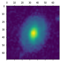
We will start by plotting some of the galaxy images that we have loaded. Do plt.matshow(train_images_raw[0,:,:,0]) (This last :,:,0] is because there are three layers to each of these galaxies and we just want to see the first layer. We’ve actually only included this first layer for you to save space, but if you want to use the full data this is necessary)

The g band is the grayscale image. To get it to display as such, instead of using false color, you can try using cmap='gray' as an argument to matshow

#plot me here!

You should see a galaxy. Now, let’s see what this galaxy should be classified as. Go ahead and print out train_labels[0].

## print out the label

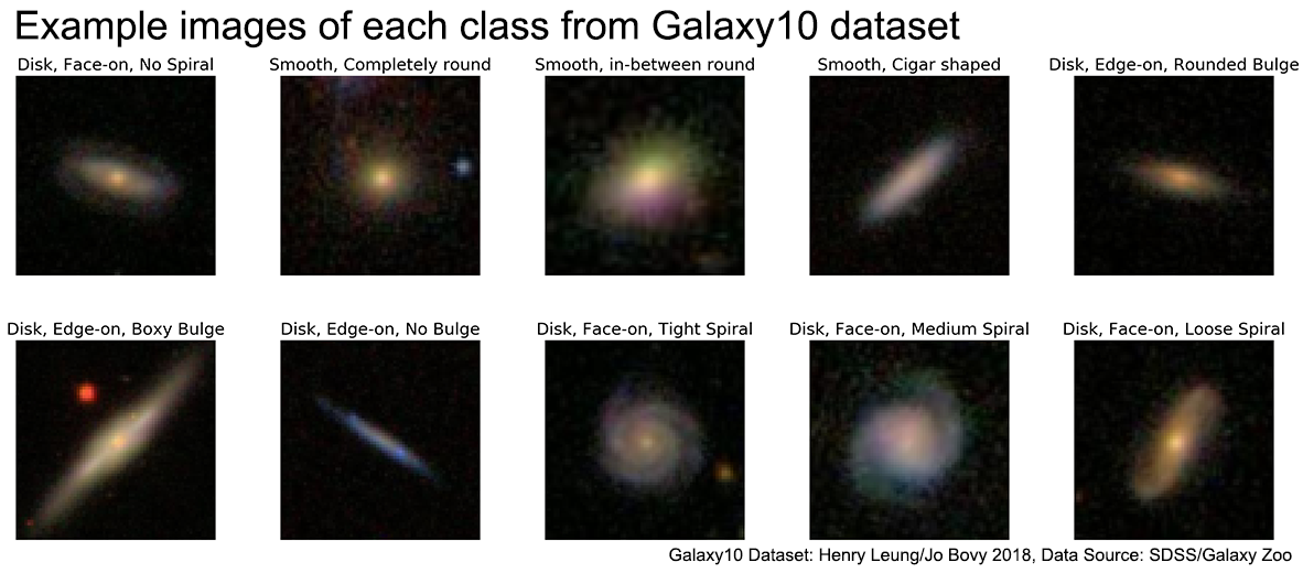
The galaxy dataset labels are given as follows. To make the exercise a little more simple, we have reduced the dataset to galaxies that are only classified as 5 of the types listed below.

Galaxy10 dataset (25753 images)

Class 0 (3461 images): Disk, Face-on, No Spiral: [1,0,0,0,0]
Class 1 (6997 images): Smooth, Completely round: [0,1,0,0,0]
Class 2 (6292 images): Smooth, in-between round: [0,0,1,0,0]
Class 3 (394 images): Smooth, Cigar shaped: skipped
Class 4 (3060 images): Disk, Edge-on, Rounded Bulge: [0,0,0,1,0]
Class 5 (17 images): Disk, Edge-on, Boxy Bulge: skipped
Class 6 (1089 images): Disk, Edge-on, No Bulge: skipped
Class 7 (1932 images): Disk, Face-on, Tight Spiral: [0,0,0,0,1]
Class 8 (1466 images): Disk, Face-on, Medium Spiral
Class 9 (1045 images): Disk, Face-on, Loose Spiral

Galaxy10 dataset

Let’s instead display the image and label for image 98. We see that instead this is a disk galaxy (this might depend on the randomness used in splitting up the training set so we need to check again when we re-pickle)

plt.matshow(train_images_raw[98,:,:,0])
print(train_labels[98])

[1. 0. 0. 0. 0.]

_images/d84158904dde5b443f140a07556e9bcbd4b5b4c682a8eb58649f68c5885a73a6.png

Let’s check the shape of our data. Go ahead and print out train_images_raw.shape

print(train_images_raw.shape)

(17457, 69, 69, 1)

We have 17457 images. Each image is a \(69 \times 69 \times 1\) image. We are going to give these pictures as inputs to our neural network. It will be easier to give them a big \(69 \times 69 \times 1 = 4761\) vector then a tensor like this. Therefore, we should go ahead and reshape our data. To do this, we can do train_images=train_images_raw.reshape(len(train_images_raw),69*69*1) (Do the same thing for our test_images_raw data). You also need to normalize the image data so it’s between 0 and 1. To do that divide all your vectors by 256

train_images = train_images_raw.reshape(train_images_raw.shape[0],69*69*1)/256.
test_images  = test_images_raw.reshape(test_images_raw.shape[0],69*69*1)/256.

We will work with these reshaped vectors for most the rest of this assignment.

b. Neural Network#

Warning: Use `jnp`!#

Notice that at the top of the file, we have imported jax.numpy as jnp alongside regular numpy as np. To proceed with this assignment, you now need to start using jnp instead of np. It’s a drop-in replacement for all functions (sum, log, etc.) that you’ll normally use in numpy but is required for the fancy gradient calculations necessary for training your net.

Our next step is to write a neural network. A neural network might sound complicated but it’s actually really simple. All our neural network does is take the input vector (our reshaped image) to an output vector (of size 5 because we have five different ways to classify a galaxy).

The equation for how to do this is \(v_{out} = 1.0/(1+\exp(-(W_2 \textrm{tanh}(W_1 v_{in} + b_1) +b_2))\) where

W1 is a size d x 4761 matrix
W2 is a size 5 x d matrix
b1 is a size d matrix
b2 is a size 5 matrix

The last term: \(1/(1+e^{-x})\) ensures that all the numbers in \(v_{out}\) are between 0 and 1.

Implement a function

def net(p,imageVector):
   a1 = p.W1@imageVector
   # other computations
   # return output

where p is a NamedTuple that contains these parameters and imageVector is one of our reshaped images.

You can define and initialize the NamedTuple as follows (keep in mind that you may need to change this):

from typing import NamedTuple

class Params(NamedTuple):
    W1: jnp.ndarray  # d x 4761
    b1: jnp.ndarray
    W2: jnp.ndarray
    b2: jnp.ndarray

d = 10
key = jax.random.PRNGKey(12423)
p = Params(W1 = 0.1*jax.random.normal(key, (d, 69*69*1)),
           b1 = jnp.zeros((d,)),
           W2 = 0.1*jax.random.normal(key, (5, d)),
           b2 = jnp.zeros(5))

You can access the variables by using p.b1 etc.

Let’s test this out. Generate a set of random parameters that have the correct dimension. Then call net(params,train_images[3]) and you should get what your current neural network guesses is the classification for the “3’rd” galaxy. Use \(d=100\).

Q: Compare your prediction to the actual classification for image 3. Is it making a good prediction? Why or why not?

A:

Notice that the output isn’t a nice vector like [0,0,0,0,1]. Instead, it has five different numbers between zero and one such as [0.2400989 , 0.39862376, 0.4565858 , 0.286503 , 0.734855 ] We will say that the neural network classifies the galaxy by whichever index is largest i.e. np.argmax(outputVector). In this case it is the 0.8866 which corresponds to spot 4 or “Disk Edge on- rounded bulge” category.

c. Measuring the quality of the model#

To quantify how good our neural network is, we will use two things:

(1) Cross-entropy Let’s quantify how far off you are from the expected label (maybe it’s [0,0,0,1,0]) . A good way to quantify this is to use the cross entropy. The cross-entropy is defined as

\[ \sum_i -y_i \log(a_i) - (1-y_i)\log(1-a_i)\]

where \(y_i\) is the \(i'\)th component of the exact label and \(a_i\) is the \(i'\)th component of the label you get as output from the neural network.

Write a function loss(params, imageVector, correctLabel) that takes the parameters and the imageVector, runs the neural network to get the output a (i.e. a=net(params,imageVector)) and then returns the cross entropy. Check the cross entropy you are getting. Our goal will be to minimize this cross entropy (if we do this, then our network will do a better job of getting the correct galaxy classification)

##

(2) Correct classification In addition to the cross-entropy, we care whether the winning labelling is correct. We will say that we’ve labelled it correctly if in our length 10 vector, the maximum value is where the 1 should be. Write a function def accuracy(params,image,label) that says whether a single image you got correct. (jnp.argmax is probably useful here). Run this on your test images and labels.

Show that your accuracy function correctly computes whether the classification is correct for one or two image examples.

Once you can compute whether a single image correctly classifies, jax makes it easy to extend it to many images. Define

fractionCorrect = jax.vmap(accuracy, in_axes = (None, 0, 0))

This makes fractionCorrect into a function, in which the second and third argument now have an extra dimension. Whereas you called accuracy as

accuracy(params, train_images[3], train_labels[3])

you will instead call fractionCorrect as

fractionCorrect(params, train_images, train_labels)

and it will return an array for all the images. You can then take the mean as jnp.mean for the fraction.

###

You probably got about 30% correct with your random values of w1,b1,w2,b2. Now we have to do better. We are going to work on getting our loss down (and this will get our fractionCorrect down). Getting the loss down is easier because it depends continuously on the parameters).

To make an objective function better, what we should do is to step in a direction where it gets better. To do this, we are going to want to get the gradient. We can use jax to get the gradient as we have in earlier assignments.

Let’s define the gradient of the loss as loss_grad = jit(jax.grad(jit(loss))). (The jit are there to make things faster. This is morally just jax.grad(loss) and that would work albeit be slower).

d. Training using stochastic gradient descent#

Now all we need to do is to (over and over again)

choose a random image in the training set.
compute the gradient
change the parameters by 0.1% of the gradient (called the learning rate \(\eta\))

This will make your result on this image marginally better.

Every 2000 steps you might want to check the fraction of your test set that is now correct. Print it out as well as push it to a list. You should find that your accuracy rises from 30% beyond 66%. Plot your accuracy as a function of step for at least 50*2000, and if patient out to 100*2000.

##

e. Testing#

By this point you should have a somewhat accurate classifier. 66% is not great for production work; you can do better by improving your training and the size of your network, but to keep the assignment reasonable we will stop there.

Now we would like to know how accurate we would expect our model to be on data it’s never seen before. You can’t use the data you trained on because your model has already seen it; we want to make sure that it’s not just memorizing the data that it’s already seen (this is sometimes referred to as overfitting). This is where the test data comes in. Use your fractionCorrect function to assess how good your model is on the test data set.

Q: Did you overfit your model? Why or why not?

A:

Acknowledgement: This assignment follows very closely a tutorial from GalaxyZoo.com

Bryan Clark and Ryan Levy (original)