
N ways to measure \(\pi\)#
Author:
Date:
Time spent on this assignment:
Remember to execute this cell to load numpy and pylab.
In this project we will consider three different ways of measuring \(\pi\).
Look for the owl emoji 🦉 for instructions
Exercise 1: Series#
List of collaborators:
References you used in developing your code:
In this exercise we will compute the value of \(\pi\) using a series (a sum of bunch of terms). We will use different series which converge at different rates.
a. \(\pi\) from \(\tan\)#
Recall that we can generally find infinite series representations of transcendental functions like \(\sin(x)\). In particular
Since \(\tan^{-1}(1) = \pi/4\), we can write the following (slowly converging) infinite series:
If we group adjacent terms in the series we can rewrite this as
The value of \(\pi\) is \(3.14159265358979323846264338327950288419716939937510582...\) though the precision with which your computer can calculate it is probably limited to fewer digits than this.
🦉Please write a Python script that calculates an approximation to \(\pi\) using the arctan series i.e. the boxed formula, and compare its accuracy after the \(n = 10\) term, 100 term, 10,000 term, and 1,000,000 term. To compare its accuracy, print out (after those three terms) the value and the difference from \(\pi\).
There are two ways to approach this. One of these is by writing a loop (use a conditional statement to print something after the appropriate terms):
Start by initializing a few things, then executing a loop that calculates the nth term, with n running from 0 to 999,999, summing the terms as you go.
The other option is to write this in a line or two using list comprehensions.
Let us start with a loop.
sum as a variable! Notice how
sum is green in a cell - this means it is a special keyword.Write your for loop computing the difference from \(\pi\) for a given term in the series below.

# ANSWER ME

b. List Comprehensions#
We’ll now look deeper at the terms in the series above, in order to practice plotting and analyzing data.
Recall that we can store items into a list. A very useful feature about a list is that it can be variable length!
To initialize a new list we use [], and can add to it by using the append() function
myList = []
myList.append(10)
print(myList)
print("myList is length",len(myList))
[10]
myList is length 1
This is obviously most useful in a for loop, where we can append numbers to the list.
myList = [] #don't forget to reset it!
for i in range(0,5):
    myList.append(i+5)
print(myList)
print("myList is length",len(myList))
[5, 6, 7, 8, 9]
myList is length 5
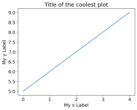
We’ll want to plot some lists in a moment. Plotting things in python uses the matplotlib package, imported as plt. There are two basic steps for plotting:
plt.plot(x,y)This tells matplotlib to plot the lists or arrays
xandy. You can also add instructions on how it should look after x,y. If we wanted a dashed line we can useplt.plot(x,y,'--')or if we want square points we can useplt.plot(x,y,'s')
plt.show()This tells matplotlib you’re done drawing/adding data and to render the image
#if we add '--' it will be dashed, and if we add 's' there will be squares. What if we do both?
plt.plot(range(0,5),myList)
plt.xlabel("My x Label")
plt.ylabel("My y Label")
plt.title("Title of the coolest plot")
plt.show()
🦉 Make a list piList which contains the terms
in the \(\tan^{-1}\) series above.
Now we need to evaluate the cumulative sum of piList, which can be done using piList_cumulative = np.cumsum(np.array(piList))
Now we want to graph the difference from \(\pi\). Go ahead and graph
plt.plot(np.abs(np.pi-piList_cumulative))
You’ll probably find that the terms in the series get very small very quickly! To see them a little better we can adjust the y-axis to be scalled logarithmically rather than linearly, by calling plt.yscale('log').
Make sure you label your axis!
Start by initializing a few things, then executing a loop that calculates the nth term, with n running from 0 to 999,999, summing the terms as you go.
Write your code (and generate your plot) below.
#ANSWER ME
c. \(\pi\) from Ramanujan#
A much more rapidly converging series was discovered by the brilliant Indian mathematician Srinivasa Ramanujan. It is
where \(k!\) (“k factorial”) is \(1\times 2\times 3\times ... \times k\) and \((4k)!\) is \(1\times2\times3\times ... \times 4k\)
🦉Write a Python script that calculates an approximation to \(\pi\) using the Ramanujan series, and comment on its accuracy after 1, 2, and 3 terms. (Recall that the value of \(\pi\) is 3.14159265358979323846264338327950288419716939937510582…)
Note that there are even faster-converging formulas than this! One, mentioned in Wolfram MathWorld1, adds 50 digits of precision for each additional term.
Please put your loop showing your approximation to \(\pi\) below again plotting (on a log-scale) the difference from \(\pi\).
You might only get the \(k=0\) and \(k=1\) term on your plot because of how quickly the series converges.
# ANSWER ME
Exercise 2: Archimedes#
List of collaborators:
References you used in developing your code:
Archimedes was an ancient greek who lived in 287 BC (wikipedia). He developed a way to approximate \(\pi\) by estimating the circumference of the circle \(C\) of known radius \(r\) by a series of polygons inscribed within the circle. Once we know the circumference, \(C=2\pi r\) and therefore \(\pi = C/(2r)\).
Note: don’t worry about using \(\pi\) in your code below!
a. Drawing a circle#
🦉Start by defining a function DrawCircle() which plots a circle (but don’t call plt.show() at the end of it.) You can then generate your circle by doing
DrawCircle()
plt.axis('scaled') # this makes your circle look like a circle and not an oval
plt.show()
Recall that the for a circle of radius \(r\),
\(x=r\cos\theta \hspace{2cm} y=r\sin\theta\)
where \(0 \leq \theta \leq 2\pi\). Plot all points starting with \(\theta=0\) with increments of \(d\theta=0.0001\) until you get to \(2\pi\). In this problem, we will work with a circle of radius \(r=1\).
Draw your circle below!
# ANSWER ME
b. Drawing a polygon#
🦉Now that you can draw a circle, the next step is to draw a polygon inside the circle. Write a function DrawPolygon(N). The points of a \(N\)-sided polygon should be at angles \(2\pi/N\). You should add an extra point at the end so your polygon looks closed.
Use your function to draw a 5-sided polygon (after drawing the circle):
DrawCircle()
DrawPolygon(5)
plt.axis('scaled') # this makes your circle look like a circle and not an oval
plt.show()
Write below your function to draw a \(N\) sided polygon and then use it to draw a 5-sided polygon. You can use dTheta = 2*np.pi/N in your function.
# ANSWER ME
c. Python Fun - List Comprehensions#
A cool Python feature is list comprehensions. Instead of writing a for loop, if we’re clever we can stuff everything into one line inside a list, and python will be able to fill out the list faster than doing an append().
Check out the example below:
slowList = []
for i in range(0,5):
    slowList.append(i-5)
# now we rearrange the syntax, so what we want each element to be
# is *first* and the for loop statement is after
fastList = [i-5 for i in range(0,5)]
print("slowList=",slowList)
print("fastList=",fastList)
slowList= [-5, -4, -3, -2, -1]
fastList= [-5, -4, -3, -2, -1]
🦉Rewrite your answer to b. to use list comprehensions, turning any for loops you had into one line.
You can have a function that generates all the x points in one line and all the y points in another line.
# answer here!
🦉 Now modify your function above to return the perimeter (divided by 2) of the polygon that you drew.
Report how close is your answer to \(\pi\) for \(N=100\).
Plot the percentage error estimate of \(\pi\) i.e. (est-truth)/truth*100, from a \(N\)-sided polygon as a function of \(3<N\leq100\).
Use plt.axhline(0,linestyle='--') to draw a line where \(\pi\) is on your plot.
# ANSWER HERE
d. Inscribed Polygon (EC) (Extra Credit: 5 points)#
Do the same thing you did earlier but use both the inscribed and circumscribed polygons. On your plot, you should see that you approach \(\pi\) from above and below.
# ANSWER HERE
Exercise 3: Throwing Darts#
List of collaborators:
References you used in developing your code:
In this exercise, we will compute \(\pi\) by (in silico2) throwing darts at a board. To do this, we are going to need to use random numbers.
You can read about Python’s (pseudo)random number generating functions here. They live in the random library, and can be imported using import random. Here’s a snippet of code that generates a sequence of random numbers between -1 and 1.
import random
for i in range(1,10):
    print(random.uniform(-1,1))
-0.11688000201076276
0.03620220098787574
0.2883853548821864
0.6498082829172125
0.09791115220296942
-0.08924271820141816
-0.7695799517173709
-0.6023607366894421
-0.818574038737153
A couple of fine points: uniform(-1,1) generates random numbers with a uniform distribution in the semi-open range [-1.0,1.0); the range specification in the for loop requires i to be greater than or equal to 1, but less than 10. Only nine random numbers are printed.
a. Darts at a board#
🦉Call DrawCircle() to draw a circle of radius 1.0 in a \(2 \times 2\) square. Then pick 25 random points \((x,y)\) in the square (do this by picking two random numbers each between -1 and 1). Plot them within the square (plt.scatter(x,y,marker='.',color='red'). Recall that the area of a circle is \(\pi r^2\), and that if you inscribe a circle of radius 1.0 inside a square of side length 2, the ratio of the areas of the circle and square will be \(\pi\)/4.
Because the dart is likely to hit any place on the square, the fraction of dots within the circle is the ratio of the area between the circle and the square.
I removed all the axis to make them look prettier by doing:
plt.xlim(-1,1)
plt.ylim(-1,1)
plt.gca().get_xaxis().set_visible(False)
plt.gca().get_yaxis().set_visible(False)
plt.show()
Code below for circle and random points in a square.
# ANSWER HERE
b. \(\pi\) from Darts#
🦉Within your loops, measure the fraction of dots that actually end up in your circle. Measure \(\pi\) using this number both with 25 dots as well as 2500 dots (for this latter number you might want to turn off the plotting or it will be really slow).
Code for fraction of points which are in the circle. This should be \(\pi/4\) so multiply by 4 to get \(\pi\)
# ANSWER HERE
c. Repeated Experiments#
🦉Now wrap your code in an additional outer loop which runs 1000 times. You now have an outer loops (1000 times) and inner loop (2500 times). You are now estimating \(\pi\) 1000 times.
Store each of the estimates in an array (or list) and generate a histogram (bar graph) of the values in the array using plt.hist. If my estimates were stored in a list named storedVals I can generate a histogram by
plt.hist(storedVals)
#...add axis labels, etc here...
plt.show()
Finally increase the number of iterations in your inner loop from 2,500 to 10,000. How does the width of your histogram change?
(You should find that it is about half as big. It is very common for statistical precision to improve proportional to the square root of the number of samples in your average.)
Plot your two histograms below.
# ANSWER HERE
Exercise 4: Buffon’s Needle (EC) (Extra Credit: 10 points)#
List of collaborators:
References you used in developing your code:
Read about Buffon’s needle and implement a simulation of it to get \(\pi\).
Acknowledgements:
Ex. 1,3 originally developed by George Gollin
Ex. 2 developed by Bryan Clark
© Copyright 2023
1http://mathworld.wolfram.com/PiFormulas.html
2performed by computer simulation; by silicon
Printing your submission#
Make sure you save a copy to your google drive in “Colab Notebooks”. If you save it somewhere else change the path below.
Make sure everything runs when you “Restart session and run all”.
The below code should automatically create an HTML file. You will likely need to authorize it access to your Google Drive.
Open the HTML file in any browser and print to PDF.
from requests import get
from socket import gethostname, gethostbyname
ip = gethostbyname(gethostname())
filename = get(f"http://{ip}:9000/api/sessions").json()[0]['name']
print(filename)
from google.colab import files
from google.colab import drive
drive.mount('/content/drive')
#filename = "FILE_NAME_GOES_HERE"
filepath = "/content/drive/MyDrive/Colab Notebooks/" + filename
!cp "$filepath" ./
!jupyter nbconvert --to HTML "$filename"
files.download(filename.replace("ipynb","html"))
---------------------------------------------------------------------------
ConnectionRefusedError                    Traceback (most recent call last)
File /opt/hostedtoolcache/Python/3.14.4/x64/lib/python3.14/site-packages/urllib3/connection.py:204, in HTTPConnection._new_conn(self)
    203 try:
--> 204     sock = connection.create_connection(
    205         (self._dns_host, self.port),
    206         self.timeout,
    207         source_address=self.source_address,
    208         socket_options=self.socket_options,
    209     )
    210 except socket.gaierror as e:

File /opt/hostedtoolcache/Python/3.14.4/x64/lib/python3.14/site-packages/urllib3/util/connection.py:85, in create_connection(address, timeout, source_address, socket_options)
     84 try:
---> 85     raise err
     86 finally:
     87     # Break explicitly a reference cycle

File /opt/hostedtoolcache/Python/3.14.4/x64/lib/python3.14/site-packages/urllib3/util/connection.py:73, in create_connection(address, timeout, source_address, socket_options)
     72     sock.bind(source_address)
---> 73 sock.connect(sa)
     74 # Break explicitly a reference cycle

ConnectionRefusedError: [Errno 111] Connection refused

The above exception was the direct cause of the following exception:

NewConnectionError                        Traceback (most recent call last)
File /opt/hostedtoolcache/Python/3.14.4/x64/lib/python3.14/site-packages/urllib3/connectionpool.py:787, in HTTPConnectionPool.urlopen(self, method, url, body, headers, retries, redirect, assert_same_host, timeout, pool_timeout, release_conn, chunked, body_pos, preload_content, decode_content, **response_kw)
    786 # Make the request on the HTTPConnection object
--> 787 response = self._make_request(
    788     conn,
    789     method,
    790     url,
    791     timeout=timeout_obj,
    792     body=body,
    793     headers=headers,
    794     chunked=chunked,
    795     retries=retries,
    796     response_conn=response_conn,
    797     preload_content=preload_content,
    798     decode_content=decode_content,
    799     **response_kw,
    800 )
    802 # Everything went great!

File /opt/hostedtoolcache/Python/3.14.4/x64/lib/python3.14/site-packages/urllib3/connectionpool.py:493, in HTTPConnectionPool._make_request(self, conn, method, url, body, headers, retries, timeout, chunked, response_conn, preload_content, decode_content, enforce_content_length)
    492 try:
--> 493     conn.request(
    494         method,
    495         url,
    496         body=body,
    497         headers=headers,
    498         chunked=chunked,
    499         preload_content=preload_content,
    500         decode_content=decode_content,
    501         enforce_content_length=enforce_content_length,
    502     )
    504 # We are swallowing BrokenPipeError (errno.EPIPE) since the server is
    505 # legitimately able to close the connection after sending a valid response.
    506 # With this behaviour, the received response is still readable.

File /opt/hostedtoolcache/Python/3.14.4/x64/lib/python3.14/site-packages/urllib3/connection.py:500, in HTTPConnection.request(self, method, url, body, headers, chunked, preload_content, decode_content, enforce_content_length)
    499     self.putheader(header, value)
--> 500 self.endheaders()
    502 # If we're given a body we start sending that in chunks.

File /opt/hostedtoolcache/Python/3.14.4/x64/lib/python3.14/http/client.py:1353, in HTTPConnection.endheaders(self, message_body, encode_chunked)
   1352     raise CannotSendHeader()
-> 1353 self._send_output(message_body, encode_chunked=encode_chunked)

File /opt/hostedtoolcache/Python/3.14.4/x64/lib/python3.14/http/client.py:1113, in HTTPConnection._send_output(self, message_body, encode_chunked)
   1112 del self._buffer[:]
-> 1113 self.send(msg)
   1115 if message_body is not None:
   1116
   1117     # create a consistent interface to message_body

File /opt/hostedtoolcache/Python/3.14.4/x64/lib/python3.14/http/client.py:1057, in HTTPConnection.send(self, data)
   1056 if self.auto_open:
-> 1057     self.connect()
   1058 else:

File /opt/hostedtoolcache/Python/3.14.4/x64/lib/python3.14/site-packages/urllib3/connection.py:331, in HTTPConnection.connect(self)
    330 def connect(self) -> None:
--> 331     self.sock = self._new_conn()
    332     if self._tunnel_host:
    333         # If we're tunneling it means we're connected to our proxy.

File /opt/hostedtoolcache/Python/3.14.4/x64/lib/python3.14/site-packages/urllib3/connection.py:219, in HTTPConnection._new_conn(self)
    218 except OSError as e:
--> 219     raise NewConnectionError(
    220         self, f"Failed to establish a new connection: {e}"
    221     ) from e
    223 sys.audit("http.client.connect", self, self.host, self.port)

NewConnectionError: HTTPConnection(host='10.1.0.246', port=9000): Failed to establish a new connection: [Errno 111] Connection refused

The above exception was the direct cause of the following exception:

MaxRetryError                             Traceback (most recent call last)
File /opt/hostedtoolcache/Python/3.14.4/x64/lib/python3.14/site-packages/requests/adapters.py:645, in HTTPAdapter.send(self, request, stream, timeout, verify, cert, proxies)
    644 try:
--> 645     resp = conn.urlopen(
    646         method=request.method,
    647         url=url,
    648         body=request.body,
    649         headers=request.headers,
    650         redirect=False,
    651         assert_same_host=False,
    652         preload_content=False,
    653         decode_content=False,
    654         retries=self.max_retries,
    655         timeout=timeout,
    656         chunked=chunked,
    657     )
    659 except (ProtocolError, OSError) as err:

File /opt/hostedtoolcache/Python/3.14.4/x64/lib/python3.14/site-packages/urllib3/connectionpool.py:841, in HTTPConnectionPool.urlopen(self, method, url, body, headers, retries, redirect, assert_same_host, timeout, pool_timeout, release_conn, chunked, body_pos, preload_content, decode_content, **response_kw)
    839     new_e = ProtocolError("Connection aborted.", new_e)
--> 841 retries = retries.increment(
    842     method, url, error=new_e, _pool=self, _stacktrace=sys.exc_info()[2]
    843 )
    844 retries.sleep()

File /opt/hostedtoolcache/Python/3.14.4/x64/lib/python3.14/site-packages/urllib3/util/retry.py:535, in Retry.increment(self, method, url, response, error, _pool, _stacktrace)
    534     reason = error or ResponseError(cause)
--> 535     raise MaxRetryError(_pool, url, reason) from reason  # type: ignore[arg-type]
    537 log.debug("Incremented Retry for (url='%s'): %r", url, new_retry)

MaxRetryError: HTTPConnectionPool(host='10.1.0.246', port=9000): Max retries exceeded with url: /api/sessions (Caused by NewConnectionError("HTTPConnection(host='10.1.0.246', port=9000): Failed to establish a new connection: [Errno 111] Connection refused"))

During handling of the above exception, another exception occurred:

ConnectionError                           Traceback (most recent call last)
Cell In[18], line 4
      1 from requests import get
      2 from socket import gethostname, gethostbyname
      3 ip = gethostbyname(gethostname())
----> 4 filename = get(f"http://{ip}:9000/api/sessions").json()[0]['name']
      5 print(filename)
      6 from google.colab import files
      7 from google.colab import drive

File /opt/hostedtoolcache/Python/3.14.4/x64/lib/python3.14/site-packages/requests/api.py:73, in get(url, params, **kwargs)
     62 def get(url, params=None, **kwargs):
     63     r"""Sends a GET request.
     64
     65     :param url: URL for the new :class:`Request` object.
   (...)     70     :rtype: requests.Response
     71     """
---> 73     return request("get", url, params=params, **kwargs)

File /opt/hostedtoolcache/Python/3.14.4/x64/lib/python3.14/site-packages/requests/api.py:59, in request(method, url, **kwargs)
     55 # By using the 'with' statement we are sure the session is closed, thus we
     56 # avoid leaving sockets open which can trigger a ResourceWarning in some
     57 # cases, and look like a memory leak in others.
     58 with sessions.Session() as session:
---> 59     return session.request(method=method, url=url, **kwargs)

File /opt/hostedtoolcache/Python/3.14.4/x64/lib/python3.14/site-packages/requests/sessions.py:592, in Session.request(self, method, url, params, data, headers, cookies, files, auth, timeout, allow_redirects, proxies, hooks, stream, verify, cert, json)
    587 send_kwargs = {
    588     "timeout": timeout,
    589     "allow_redirects": allow_redirects,
    590 }
    591 send_kwargs.update(settings)
--> 592 resp = self.send(prep, **send_kwargs)
    594 return resp

File /opt/hostedtoolcache/Python/3.14.4/x64/lib/python3.14/site-packages/requests/sessions.py:706, in Session.send(self, request, **kwargs)
    703 start = preferred_clock()
    705 # Send the request
--> 706 r = adapter.send(request, **kwargs)
    708 # Total elapsed time of the request (approximately)
    709 elapsed = preferred_clock() - start

File /opt/hostedtoolcache/Python/3.14.4/x64/lib/python3.14/site-packages/requests/adapters.py:678, in HTTPAdapter.send(self, request, stream, timeout, verify, cert, proxies)
    674     if isinstance(e.reason, _SSLError):
    675         # This branch is for urllib3 v1.22 and later.
    676         raise SSLError(e, request=request)
--> 678     raise ConnectionError(e, request=request)
    680 except ClosedPoolError as e:
    681     raise ConnectionError(e, request=request)

ConnectionError: HTTPConnectionPool(host='10.1.0.246', port=9000): Max retries exceeded with url: /api/sessions (Caused by NewConnectionError("HTTPConnection(host='10.1.0.246', port=9000): Failed to establish a new connection: [Errno 111] Connection refused"))