Building a Physical Qubit

Building a Physical Qubit#

Author:
Date:
Time spent on this assignment:

!pip install qiskit[visualization];
!pip install qutip
!pip install qiskit_aer;

Show code cell output Hide code cell output

Requirement already satisfied: qiskit[visualization] in /opt/hostedtoolcache/Python/3.10.17/x64/lib/python3.10/site-packages (2.0.0)
Requirement already satisfied: rustworkx>=0.15.0 in /opt/hostedtoolcache/Python/3.10.17/x64/lib/python3.10/site-packages (from qiskit[visualization]) (0.16.0)
Requirement already satisfied: numpy<3,>=1.17 in /opt/hostedtoolcache/Python/3.10.17/x64/lib/python3.10/site-packages (from qiskit[visualization]) (2.2.5)
Requirement already satisfied: scipy>=1.5 in /opt/hostedtoolcache/Python/3.10.17/x64/lib/python3.10/site-packages (from qiskit[visualization]) (1.15.2)
Requirement already satisfied: sympy>=1.3 in /opt/hostedtoolcache/Python/3.10.17/x64/lib/python3.10/site-packages (from qiskit[visualization]) (1.14.0)
Requirement already satisfied: dill>=0.3 in /opt/hostedtoolcache/Python/3.10.17/x64/lib/python3.10/site-packages (from qiskit[visualization]) (0.4.0)
Requirement already satisfied: python-dateutil>=2.8.0 in /opt/hostedtoolcache/Python/3.10.17/x64/lib/python3.10/site-packages (from qiskit[visualization]) (2.9.0.post0)
Requirement already satisfied: stevedore>=3.0.0 in /opt/hostedtoolcache/Python/3.10.17/x64/lib/python3.10/site-packages (from qiskit[visualization]) (5.4.1)
Requirement already satisfied: typing-extensions in /opt/hostedtoolcache/Python/3.10.17/x64/lib/python3.10/site-packages (from qiskit[visualization]) (4.13.2)
Requirement already satisfied: symengine<0.14,>=0.11 in /opt/hostedtoolcache/Python/3.10.17/x64/lib/python3.10/site-packages (from qiskit[visualization]) (0.13.0)
Requirement already satisfied: matplotlib>=3.3 in /opt/hostedtoolcache/Python/3.10.17/x64/lib/python3.10/site-packages (from qiskit[visualization]) (3.10.1)
Requirement already satisfied: pydot in /opt/hostedtoolcache/Python/3.10.17/x64/lib/python3.10/site-packages (from qiskit[visualization]) (3.0.4)
Requirement already satisfied: Pillow>=4.2.1 in /opt/hostedtoolcache/Python/3.10.17/x64/lib/python3.10/site-packages (from qiskit[visualization]) (11.2.1)
Requirement already satisfied: pylatexenc>=1.4 in /opt/hostedtoolcache/Python/3.10.17/x64/lib/python3.10/site-packages (from qiskit[visualization]) (2.10)
Requirement already satisfied: seaborn>=0.9.0 in /opt/hostedtoolcache/Python/3.10.17/x64/lib/python3.10/site-packages (from qiskit[visualization]) (0.13.2)
Requirement already satisfied: contourpy>=1.0.1 in /opt/hostedtoolcache/Python/3.10.17/x64/lib/python3.10/site-packages (from matplotlib>=3.3->qiskit[visualization]) (1.3.2)
Requirement already satisfied: cycler>=0.10 in /opt/hostedtoolcache/Python/3.10.17/x64/lib/python3.10/site-packages (from matplotlib>=3.3->qiskit[visualization]) (0.12.1)
Requirement already satisfied: fonttools>=4.22.0 in /opt/hostedtoolcache/Python/3.10.17/x64/lib/python3.10/site-packages (from matplotlib>=3.3->qiskit[visualization]) (4.57.0)
Requirement already satisfied: kiwisolver>=1.3.1 in /opt/hostedtoolcache/Python/3.10.17/x64/lib/python3.10/site-packages (from matplotlib>=3.3->qiskit[visualization]) (1.4.8)
Requirement already satisfied: packaging>=20.0 in /opt/hostedtoolcache/Python/3.10.17/x64/lib/python3.10/site-packages (from matplotlib>=3.3->qiskit[visualization]) (25.0)
Requirement already satisfied: pyparsing>=2.3.1 in /opt/hostedtoolcache/Python/3.10.17/x64/lib/python3.10/site-packages (from matplotlib>=3.3->qiskit[visualization]) (3.2.3)

Requirement already satisfied: six>=1.5 in /opt/hostedtoolcache/Python/3.10.17/x64/lib/python3.10/site-packages (from python-dateutil>=2.8.0->qiskit[visualization]) (1.17.0)
Requirement already satisfied: pandas>=1.2 in /opt/hostedtoolcache/Python/3.10.17/x64/lib/python3.10/site-packages (from seaborn>=0.9.0->qiskit[visualization]) (2.2.3)

Requirement already satisfied: pytz>=2020.1 in /opt/hostedtoolcache/Python/3.10.17/x64/lib/python3.10/site-packages (from pandas>=1.2->seaborn>=0.9.0->qiskit[visualization]) (2025.2)
Requirement already satisfied: tzdata>=2022.7 in /opt/hostedtoolcache/Python/3.10.17/x64/lib/python3.10/site-packages (from pandas>=1.2->seaborn>=0.9.0->qiskit[visualization]) (2025.2)
Requirement already satisfied: pbr>=2.0.0 in /opt/hostedtoolcache/Python/3.10.17/x64/lib/python3.10/site-packages (from stevedore>=3.0.0->qiskit[visualization]) (6.1.1)
Requirement already satisfied: setuptools in /opt/hostedtoolcache/Python/3.10.17/x64/lib/python3.10/site-packages (from pbr>=2.0.0->stevedore>=3.0.0->qiskit[visualization]) (65.5.0)
Requirement already satisfied: mpmath<1.4,>=1.1.0 in /opt/hostedtoolcache/Python/3.10.17/x64/lib/python3.10/site-packages (from sympy>=1.3->qiskit[visualization]) (1.3.0)

Requirement already satisfied: qutip in /opt/hostedtoolcache/Python/3.10.17/x64/lib/python3.10/site-packages (5.1.1)
Requirement already satisfied: numpy>=1.22 in /opt/hostedtoolcache/Python/3.10.17/x64/lib/python3.10/site-packages (from qutip) (2.2.5)
Requirement already satisfied: scipy>=1.9 in /opt/hostedtoolcache/Python/3.10.17/x64/lib/python3.10/site-packages (from qutip) (1.15.2)
Requirement already satisfied: packaging in /opt/hostedtoolcache/Python/3.10.17/x64/lib/python3.10/site-packages (from qutip) (25.0)

Requirement already satisfied: qiskit_aer in /opt/hostedtoolcache/Python/3.10.17/x64/lib/python3.10/site-packages (0.17.0)
Requirement already satisfied: qiskit>=1.1.0 in /opt/hostedtoolcache/Python/3.10.17/x64/lib/python3.10/site-packages (from qiskit_aer) (2.0.0)
Requirement already satisfied: numpy>=1.16.3 in /opt/hostedtoolcache/Python/3.10.17/x64/lib/python3.10/site-packages (from qiskit_aer) (2.2.5)
Requirement already satisfied: scipy>=1.0 in /opt/hostedtoolcache/Python/3.10.17/x64/lib/python3.10/site-packages (from qiskit_aer) (1.15.2)
Requirement already satisfied: psutil>=5 in /opt/hostedtoolcache/Python/3.10.17/x64/lib/python3.10/site-packages (from qiskit_aer) (7.0.0)
Requirement already satisfied: rustworkx>=0.15.0 in /opt/hostedtoolcache/Python/3.10.17/x64/lib/python3.10/site-packages (from qiskit>=1.1.0->qiskit_aer) (0.16.0)
Requirement already satisfied: sympy>=1.3 in /opt/hostedtoolcache/Python/3.10.17/x64/lib/python3.10/site-packages (from qiskit>=1.1.0->qiskit_aer) (1.14.0)
Requirement already satisfied: dill>=0.3 in /opt/hostedtoolcache/Python/3.10.17/x64/lib/python3.10/site-packages (from qiskit>=1.1.0->qiskit_aer) (0.4.0)
Requirement already satisfied: python-dateutil>=2.8.0 in /opt/hostedtoolcache/Python/3.10.17/x64/lib/python3.10/site-packages (from qiskit>=1.1.0->qiskit_aer) (2.9.0.post0)
Requirement already satisfied: stevedore>=3.0.0 in /opt/hostedtoolcache/Python/3.10.17/x64/lib/python3.10/site-packages (from qiskit>=1.1.0->qiskit_aer) (5.4.1)
Requirement already satisfied: typing-extensions in /opt/hostedtoolcache/Python/3.10.17/x64/lib/python3.10/site-packages (from qiskit>=1.1.0->qiskit_aer) (4.13.2)
Requirement already satisfied: symengine<0.14,>=0.11 in /opt/hostedtoolcache/Python/3.10.17/x64/lib/python3.10/site-packages (from qiskit>=1.1.0->qiskit_aer) (0.13.0)
Requirement already satisfied: six>=1.5 in /opt/hostedtoolcache/Python/3.10.17/x64/lib/python3.10/site-packages (from python-dateutil>=2.8.0->qiskit>=1.1.0->qiskit_aer) (1.17.0)
Requirement already satisfied: pbr>=2.0.0 in /opt/hostedtoolcache/Python/3.10.17/x64/lib/python3.10/site-packages (from stevedore>=3.0.0->qiskit>=1.1.0->qiskit_aer) (6.1.1)
Requirement already satisfied: setuptools in /opt/hostedtoolcache/Python/3.10.17/x64/lib/python3.10/site-packages (from pbr>=2.0.0->stevedore>=3.0.0->qiskit>=1.1.0->qiskit_aer) (65.5.0)
Requirement already satisfied: mpmath<1.4,>=1.1.0 in /opt/hostedtoolcache/Python/3.10.17/x64/lib/python3.10/site-packages (from sympy>=1.3->qiskit>=1.1.0->qiskit_aer) (1.3.0)

import numpy as np
import matplotlib.pyplot as plt
import random
import pylab as plt
import scipy.linalg
import matplotlib.animation as animation
from IPython.display import HTML

import qiskit
import qutip
from qiskit import QuantumCircuit, transpile
from qiskit_aer import AerSimulator



def resetMe(keepList=[]):
    ll=%who_ls
    keepList=keepList+['resetMe','np','plt','random']
    for iiii in keepList:
        if iiii in ll:
            ll.remove(iiii)
    for iiii in ll:
        jjjj="^"+iiii+"$"
        %reset_selective -f {jjjj}
    ll=%who_ls
    return
import datetime;datetime.datetime.now()


def AddCircuits(theCircuits):
  numQubits=np.array([c.num_qubits for c in theCircuits])
  numQubits=np.max(numQubits)
  circuit=QuantumCircuit(numQubits,numQubits)
  for i in range(0,len(theCircuits)):
    circuit=circuit.compose(theCircuits[i],qubits=list(range(0,theCircuits[i].num_qubits)))
  return circuit


def RunMe(circuit,a=None):
  numQubits=circuit.num_qubits
  if a!=None:
    numQubits=max(numQubits,a.num_qubits)
    initCircuit=QuantumCircuit(a.num_qubits,a.num_qubits)
    initCircuit.initialize(a)
    circuit=AddCircuits([initCircuit,circuit])
  circuit.save_statevector(label='myStateVector')
  compiled_circuit = transpile(circuit, simulator)
  resultA = simulator.run(compiled_circuit).result()
  forward=list(range(0,numQubits))
  reverse=forward[::-1]
  circuit.measure(forward,reverse)
  compiled_circuit = transpile(circuit, simulator)
  resultB = simulator.run(compiled_circuit).result()
  return resultA.data()['myStateVector'],resultB.data()['counts']


def MakeState(v):
  numWires=int(round(np.log2(len(np.array(v)))))
  qc1=QuantumCircuit(numWires,numWires)
  qc1.initialize(v)
  a,_=RunMe(qc1)
  return a

def PlotBloch(v,bb):
  vv=np.asarray(v)
  a=vv[0]*np.conj(vv[0])
  b=vv[1]*np.conj(vv[0])
  x = np.real(2.0 * b.real)
  y = np.real(2.0 * b.imag)
  z = np.real(2.0 * a - 1.0)
  bb.add_vectors([x,y,z])
  return

simulator = AerSimulator()

Overview#

So far we’ve learned about quantum computing as an abstract model of computation. We can represent a qubit as a vector of length 2 (and can represent $n$ qubits as a vector of length $2^n$). This can be implemented as a superposition of any two states of a quantum system; it’s a very general concept. If we can control how a system evolves from one state to another, we can implement the abstract gates for quantum computing.

In this section our goal is to understand how we actually build a quantum computer in the real world (and here we will only focus on 1 qubit).

Our goal will be to understand how you represent one qubit and apply a gate to it.

There are various different physical realizations of a qubit. In this assignment, we will look at an infinite square well (which is easy to understand but not realistic) and quantum electronic circuits, which are currently a leading candidate for actual implementation of quantum computation.

Exericise 0: What Abstract Gate are you trying to implement?#

a. Abstract Model of Computation#

Our target here to implement a gate using electronics. We will eventually try to implement the following gate in a realistic model of a quantum system:

circuit.rx(1./50.,0)
circuit.rz(1./50.,0)

Let’s start by implementing this in qiskit.

Run the gate $k$ times (from $0 \leq k < 400$) and graph (with two lines) the probability you would measure “0” and the probability you would measure “1” as a function of $k$.

###ANSWER HERE

The state of a single qubit is $\alpha |0\rangle + \beta |1\rangle$ where $|\alpha|^2 + |\beta|^2=1$ and $\alpha$, $\beta$ are complex numbers. We might think that we could then represent the qubit by a point $(\alpha, \beta)$ which is on a circle of radius 1. But $\alpha$ and $\beta$ are complex numbers so it’s not quite that simple - instead you can represent the qubit as a point on a sphere. This is called the Bloch sphere. (Technical point: You might think that you need four numbers to represent two complex numbers but it’s actually only three because of the normalization and relative phase).

At the moment, it’s not important that you know how to perform this mapping but to understand for every qubit there is a point that it appears on the bloch sphere.

Plot the path of this gate (iterated over and over) on the Bloch sphere using something like

b = qutip.Bloch()
for state in states[::10]:
  PlotBloch(state, b)
b.render()
b.show()

in this case, state must be a complex two-dimensional vector $[\alpha,\beta]$.

### ANSWER HERE

Exercise 1: Particle in a box#

List of collaborators:
References you used in developing your code:

We will need to begin by learning or recalling some aspects about quantum mechanics. There are three key things that you need to know about quantum mechanics:

In quantum mechanics, the “rules” of the physical system are represented by a matrix called the Hamiltonian $H$ (in many ways, the classical analogue of the energy) and the state of your system is represented by a vector $\Psi$.
If your quantum is in state $\Psi(0)$ at time 0, you can figure out what your Hamiltonian is at time $t$ by $$\Psi(t) = \exp[-i t H] \Psi(0).$$ In order to do that matrix exponential you can use

expH = scipy.linalg.expm(-1.j * H * t)

If you are going to a large time $t$, it will often make sense to break it apart into a number of $T/\delta t$ smaller time steps each of size $\delta t$. This will let you record information about your quantum state at each time step $\delta t$ - i.e. something like

for step in ts:
    psi = scipy.linalg.expm(-1.j * H * delta_t) @ psi

There are special quantum states $\Psi_i$ which don’t change in time under time evolution. These states are the eigenstates of $H$. You can get the i’th eigenstate of $H$ by doing

np.linalg.eigh(H)[1][:,i]

a. Hamiltonian for a Particle in a Box#

We can start by working with a particle in a box. Consider a particle in a box of length 20 spanning $-10 \leq x \leq 10$.

The Hamiltonian for a particle in a box is

\[ H=-\frac{\partial^2 }{\partial x^2} \]

with hard walls for any $|x|\geq 20$ outside the box.

We need to convert this into a matrix. To do that, we should know from calculus that the stencil for a second derivative is

\[ \frac{\partial^2 }{\partial x^2} \equiv \frac{f(x+\delta) - 2 f(x) + f(x-\delta)}{\delta^2} \]

We can let the rows and columns of the matrix $H$ be indexed by the values of $x$ - to get the values of $x$, we can do

L = 20
delta_x = 0.05
xs = np.arange(-L/2, L/2+delta_x, delta_x)

Then the above stencil corresponds to the matrix

\[\begin{split} H[i,j] = \begin{cases} 2/(\delta x)^2 & \text{if } i == j \\ -1/(\delta x)^2 & \text{if } \textrm{abs}(i-j)== 1\\ 0 & \text{otherwise } \end{cases} \end{split}\]

Make the Hamiltonian matrix H
diagonalize it and
plot the first four eigenstates $v_a, v_b, v_c, v_d$ You should recognize the solutions to the particle in a box.

[Note: we are using units such that $\hbar=1$ and $m=1$. This is a common computational physicists’ trick so that you don’t have to carry around tons of conversion constants.]

### ANSWER HERE

The eigenvalues for a particle in a box are quantized. They should be equal to

\[E_n = \frac{\pi^2}{L^2}n^2\]

for $n=\{1,2,...\}$.

Plot the lowest five eigen-energies and compare them against this formula (they should be close but possibly not quite on because the delta_x is too big)

### ANSWER HERE

b. Time Evolution#

Our next step will be to implement time evolution. Let us start by trying to time-evolve $v_a$ under the Hamiltonian $H$. Recall that eigenstates should be stationary, and so don’t evolve in time except for an overall phase. Therefore, under time evolution we should find that this state always looks the same. Let’s check this.

Using

a total time of $T=5$
a time step of $\delta t=0.1$

Plot the value of $|v(t)|$ at time steps $t=\{0,1,3,5\}$. The absolute value is necessary because under time-evolution the wave function can become complex. You could also plot the phase of the wave function if desired but don’t worry about this.

### ANSWER HERE

You should have noticed that our previous time evolution was pretty uninteresting as nothing changed under the time evolution. Our next step will be to implement time evolution on a more complicated state.

We will consider two states that are NOT energy eigenstates:

\[v_0=\frac{1}{\sqrt{2}}(v_a+v_b)\]

\[v_1=\frac{1}{\sqrt{2}}(v_a-v_b)\]

These two states are orthogonal on each other - i.e. np.vdot(v0,v1)=0. You can check this.

We want to do time evolution with our Hamiltonian on the state $v_0$.
Perform time evolution

starting at $v_0$
$\delta t=0.1$
for time $T=50$
and graph the result at $T=\{4.0,18.3,41.0\}$
Also graph (with dotted lines - linestyle="--") $v_0$ and $v_1$

### ANSWER HERE

c. State overlaps#

We’ve seen that our time evolution slowly moves us from state $v_0$ to state $v_1$ over a time over a time of $T=41$. In between, $T=0$ and $T=41$, the state is a little bit of $v_0$ and a little bit of $v_1$. We would like to quantify this better by computing the overlap with these two states as a function of time.

We have a state $v(t)$. To compute the overlap with $v_0$ we can just do np.vdot(v , v_0).

This overlap is a complex number. We can only plot real numbers so if we want to plot it, we need to plot something like

the absolute value np.abs(...) (or its square) and
phase np.angle(...) or

Plot as a function of time from $T=0$ to $T=100$ the absolute value squared of the overlap of $v(t)$ with both $v_0$ and $v_1$.

### ANSWER HERE

Now we can get our first inkling of how you might build a qubit and a (always-on and hence not-very-useful) gate.

Suppose someone comes to you with a particle in a box. There are many eigenstates for that particle in the box: $v_0, v_1, v_2, v_3, ...$

You pick two of those eigenstates (let’s say $v_0$ and $v_1$) and label those states as $|0\rangle$ and $|1\rangle$.

This particle in a box is now a qubit. The other eigenstates we ignore and try to make sure that you never accidentally end up in - this would cause an error if so.

Now a gate is something that takes you from one quantum state to another. For example, a not gate should take

\[|0\rangle \rightarrow |1\rangle\]

\[|1\rangle \rightarrow |0\rangle\]

Looking at our previous results, we can see that if we just have a particle in a box that it implements a not-gate every $T=41.0$ seconds.

In principle this would work as a qbit; however, it is difficult to set up in practice. The closest thing we have to particles in boxes are so-called quantum dots, and it is difficult to prepare a state in superposition like we did above, and even if we did, we could not easily apply the potential energy for well-controlled amounts of time. We really need a Hamiltonian $H(\theta)$ where we have some knob $\theta$ that we can change so we can turn gates on and off.

In the next exercise, we will see how to go about this.

Exercise 2: Fluxonium#

In this exercise, we will work a large system built out of electronic circuits that we can control well. This particular setup is called fluxonium, because it looks a little like an atom that we can control using a magnetic flux.

Here is the electronic circuit for a fluxonium qubit:

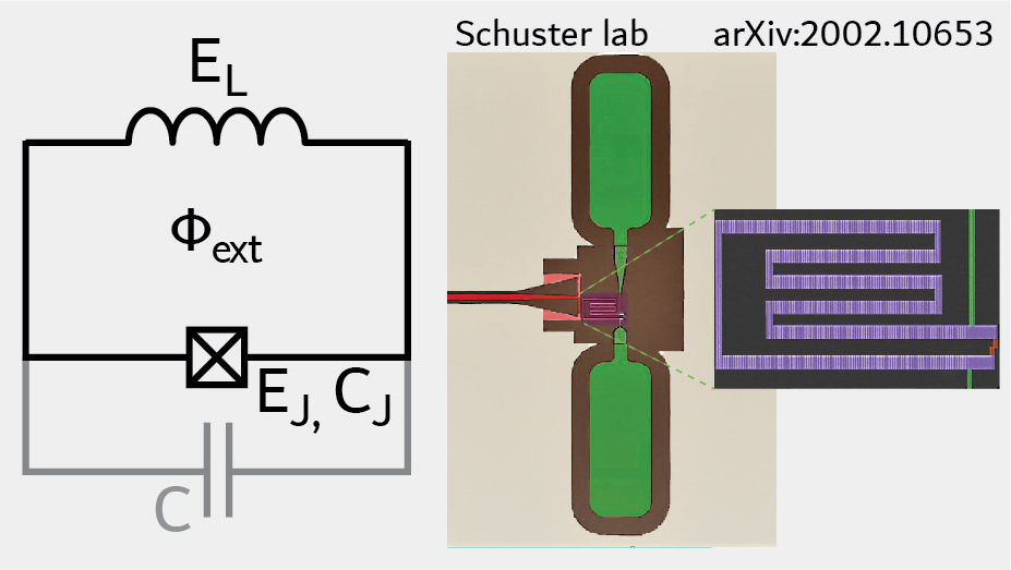
The fluxoinum qubit consists of three electronic components: a capacitor, an inductor, and a Josephson junction. You’re probably familiar with capacitors and inductors. You regularly run into them in classical circuits. A Josephson junction is an electronic component that sandwiches an insulator between two superconducting materials. Across the Josephson junction there is a change in the phase $\phi$, which is our quantum variable. This $\phi$ roughly corresponds to the current. If you recall from quantum mechanics, the momentum of a particle is related to its phase change across space; the same is true here for current.

Typically in a circuit you need to keep track of the voltage and current. When you have a Josephson junction you need to keep track also of the phase.

In electronics you might have treated the circuit classically - i.e. $E=\frac{1}{2}CV^2+ \frac{1}{2}LI^2$ We are basically doing this in writing out the Hamiltonian, except we will write it in terms of the variable $\phi$, the phase difference across the Josephson junction. These circuits are kept extremely cold, on the order of milliKelvin, and are reasonably small that they need a fully quantum description, even though they are made up of many electrons and nuclei.

a. Fluxonium Hamiltonian#

The relevant Hamiltonian for fluxonium is

\[H=-4E_\text{C}\frac{\partial^2 }{\partial \phi^2}+\frac{1}{2}E_L \phi^2 -E_\text{J}\cos(\phi-\varphi_\text{ext}) \]

where $E_C$ is the charging energy, $E_J$ the Josephson energy and $E_L$ the inductive energy.

In the particle in a box we were working with $x$. Here you could just mentally replace $\phi$ with $x$. Just like earlier we will let $-10\leq \phi \leq 10$.

Now we can look at this Hamiltonian. The first term, $-4E_\text{C}\frac{\partial^2 }{\partial \phi^2}$ you’ve already seen; this is the particle in a box term (notice the extra factor of $4E_C$). You already know how to build the matrix for this term. This term is caused by the capacitor. Essentially the capacitor would like the wave function (when drawn in the $\phi$ basis) to be more spread out.

We will then need to add a matrix for the the inductor term and the Josephson junction term. Both of these terms will be diagonal matrices.

The term $\frac{1}{2}E_L \phi^2$ is the Hamiltonian for the inductor and has the matrix $H[\phi,\phi] = \frac{1}{2}E_L \phi^2$ (and zero otherwise)

The term $E_\text{J}\cos(\phi-\varphi_\text{ext})$ is the Hamiltonian for the inductor and has the matrix $H[\phi,\phi] = E_\text{J}\cos(\phi-\varphi_\text{ext})$ (and zero otherwise).

$\varphi_\text{ext}$ is a number that you (as an experimentalist) get to control as a knob. It corresponds to the amount of magnetic flux (caused by sticking a magnet in the right place) you drive through the circuit loop. Classically you know that a changing magnetic field can induce a current, similarly here it can affect $\phi$.

By changing the magnetic field we will be able to control the quantum state of the circuit.

Build this Hamiltonian for $H$. Use the following parameters:

Ec=0.5
El=0.8
Ej=4
$\varphi_\text{ext}=\pi$

The units here are set up such that the time evolution is in seconds later.

As in the previous case, we want to diagonalize our Hamiltonian and find some number of eigenstates. Plot the first three eigenstates as well as eigenvalues.

### ANSWER HERE

b. Time Evolution#

We are going to use the first two eigenstates for $\varphi_{ext}=\pi$: $v_0$ and $v_1$ as the $|0\rangle$ and $|1\rangle$ states for our qubit. Then we are going to see how manipulating $\varphi_\textrm{ext}$ allows us to turn on and off different gates. Note that our definition of $|0\rangle$ and $|1\rangle$ will not change.

You should find that it begins to be a superposition $\alpha |0\rangle + \beta |1\rangle$. You can compute these as follows:

$\alpha$ = np.vdot(v0, v)
$\beta$ = np.vdot(v1,v) where v is the time-evolved state.

Begin with the state $|0\rangle$. Then change the magnetic field to $\pi + 0.00360 \times 2\pi$ and begin to time-evolve the state. Do time evolution with the new Hamiltonian for a

time $T=100$ with
$\delta t=0.1$ and
plot the overlap squared with the states $|0\rangle$ and $|1\rangle$, i.e., $|\alpha|^2$ and $|\beta|^2$

### ANSWER HERE

You will notice that by changing the magnetic field by a tiny amount and waiting for about 24 seconds, we’ve implemented a gate which takes $|0\rangle$ to half $|0\rangle$ and half $|1\rangle$. Based on the probability this gate is taking $|0\rangle \rightarrow \frac{1}{\sqrt{2}}(|0\rangle + e^{i\theta} |1\rangle)$, where $e^{i\theta}$ is a phase that you could compute by looking at the phase difference between $\alpha$ and $\beta$.

c. The Bloch Sphere#

Using your results from (b), plot the time evolution from above on the Bloch sphere. Remember that you need to pass the plotting function the $[\alpha,\beta]$ vectors. Identify where on the Bloch sphere the initial point is and the point at $T=44$ seconds. Compare the action of this operation with the gate you did at the beginning of the exercise.

### ANSWER HERE

Building a Physical Qubit

Contents

Building a Physical Qubit#

Overview#

Exericise 0: What Abstract Gate are you trying to implement?#

a. Abstract Model of Computation#

Exercise 1: Particle in a box#

a. Hamiltonian for a Particle in a Box#

b. Time Evolution#

c. State overlaps#

Exercise 2: Fluxonium#

a. Fluxonium Hamiltonian#

b. Time Evolution#

c. The Bloch Sphere#